Introduction to Key-Value Cache

This post presumes familiarity with the transformer architecture and how tokens are computed and selected. During inference, we autoregressively generate new tokens given all the previous tokens generated. At \(t=k\), we have a sequence of generated tokens

<\(\text{sos}\)>, <\(t_{1}\)>, <\(t_{2}\)>,…, <\(t_{k-1}\)>

and feed it to the transformer. We generate a new token and append it to the input sequence and give it back to the transformer to get the next token.

<\(\text{sos}\)>, <\(t_{1}\)>, <\(t_{2}\)>,…, <\(t_{k-1}\)>, <\(t_{k}\)>

The attention matrix is given by (masking is omitted for simplicity):

\[ Attention(Q, K, V) = \sigma \left[ \frac{QK^{T}}{\sqrt{d}_{k}} \right]V \]

Attention Computation

In matrix form, the attention computation is

At \(t=1\)

\[ \begin{bmatrix} q_{11} & q_{12} & ... & q_{1d} \end{bmatrix} \begin{bmatrix} k_{11} \\ k_{12} \\ ... \\ k_{1d} \end{bmatrix} = \begin{bmatrix} qk^{T}_{11} \end{bmatrix} \begin{bmatrix} v_{11} & v_{12} & ... & v_{1d} \end{bmatrix} = \begin{bmatrix} a_{11} & a_{12} & ... & a_{1d} \end{bmatrix} \]

…

At \(t=k\)

\[ \begin{bmatrix} q_{11} & q_{12} & ... & q_{1d} \\ q_{21} & q_{22} & ... & q_{2d} \\ ... \\ q_{k1} & q_{k2} & ... & q_{kd} \end{bmatrix} \begin{bmatrix} k_{11} & k_{21} & ... & k_{k1} \\ k_{12} & k_{22} & ... & k_{k2} \\ ... \\ k_{1d} & k_{2d} & ... & k_{kd} \end{bmatrix} = \begin{bmatrix} qk^{T}_{11} & qk^{T}_{12} & ... & qk^{T}_{1k} \\ qk^{T}_{21} & qk^{T}_{22} & ... & qk^{T}_{2k} \\ ... \\ qk^{T}_{k1} & qk^{T}_{k2} & ... & qk^{T}_{kk} \\ \end{bmatrix} \begin{bmatrix} v_{11} & v_{12} & ... & v_{1d} \\ v_{21} & v_{22} & ... & v_{2d} \\ ... \\ v_{k1} & v_{k2} & ... & v_{kd} \end{bmatrix} = \begin{bmatrix} a_{11} & a_{12} & ... & a_{1d} \\ a_{21} & a_{22} & ... & a_{2d} \\ ... \\ a_{k1} & a_{k2} & ... & a_{kd} \end{bmatrix} \]

Redundant Computations

Consider the Decoder Transformer Architecture:

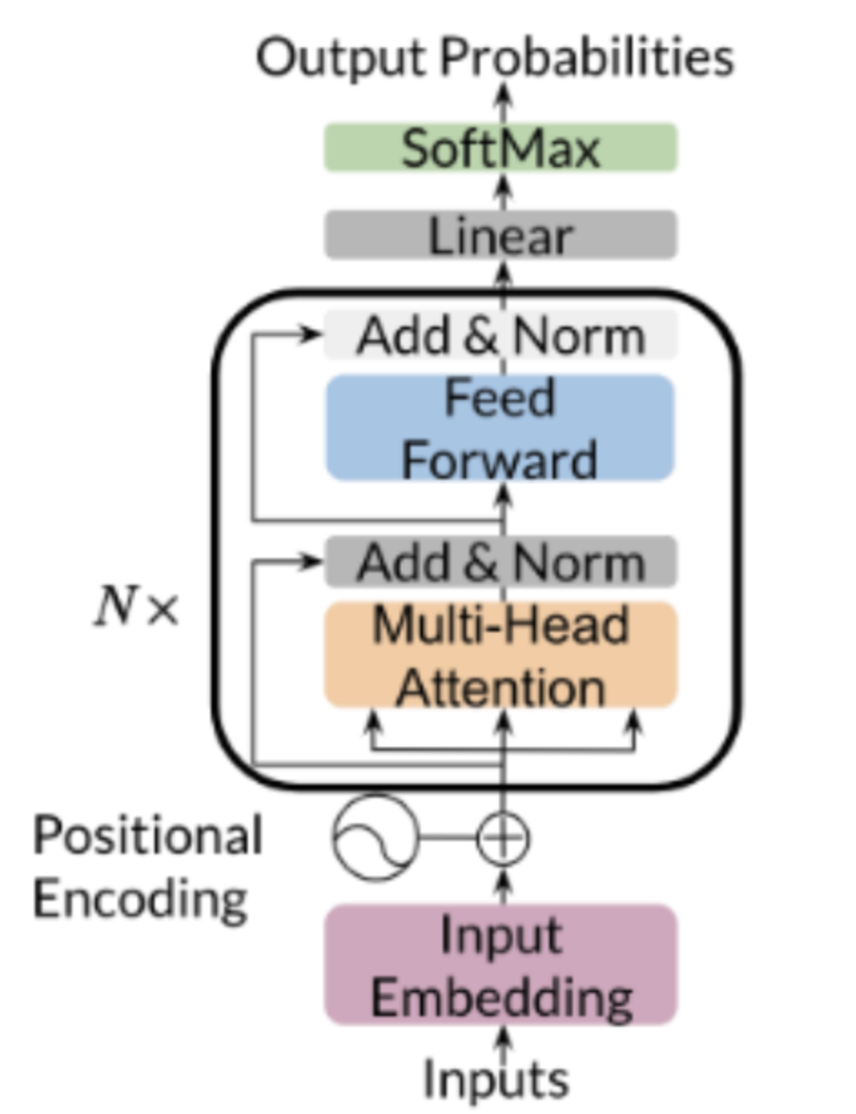
We omit the feedforward and normalisation layers to focus on the relationship between the output of the attention block and the output. The \(k \times d\) attention matrix will processed by the rest of the transformer to produce a matrix of logits.

For the next token prediction, we require only the last row of the logits matrix which will be mapped to a token and appended to the input sequence. Tracing this to the attention matrix, we also only require the final row of the \(A\) matrix, we don’t need to compute the other rows.

Consider the final (here it’s at index \(k\)) row, corresponding to the latest token of the attention matrix \(A\). It can be decomposed as

\[ \mathbf{a}_{k} = [a_{k1} a_{k2} \cdots a_{kd}] = (\mathbf{q}_{k}K^{T})V \]

where

\(k\) is the index of the latest token

\(\mathbf{q}_{k}\) is the k-th row of the query matrix \(Q\)

\(K\) and \(V\) are the full Key and Value matrices

The attention matrix is used downstream to compute the logit matrix. Simplifying the intermediate feedforward layers and assuming only 1 attention head, we get

\[ S = softmax[AW] \in \mathbb{R}^{k \times |V|}\]

where

\(|V|\) is the vocabulary size

\(A \in \mathbb{R}^{k \times d}\) is the attention matrix

\(W \in \mathbb{R}^{d \times |V|}\) is the weight matrix

To decode the latest token, we only require the final row of \(S\) - \(\mathbf{s}_{k}\). It can be decomposed as (substitute \(\mathbf{a}_{k}\) into \(\mathbf{s}_{k}\))

\[ \mathbf{s}_{k} = \mathbf{a}_{k}W = [[\mathbf{q}_{k}K^{T}]V]W \]

where

\(\mathbf{q}_{k} = \mathbf{x}_{k}W_{q}\)

\(\mathbf{x}_{k}\) is the token embedding for the most recent token.

Looking at \(\mathbf{s}_{k}\), for every token generated, we require the entire \(K, V\) matrices, they can be cached and the new vectors must be appended. The expensive projection calculations can only be computed for the single new token at each step. All historical information is preserved in the cache. For the query token, we only need the token embedding for the most recent token - \(\mathbf{x}_{k}\).

Inference loop with KV cache

At each step, instead of recomputing the entire history, the Key and Value matrices are stored. The process when generating a token is:

1. Receive new token: The model receives an embedding for the single latest token.
2. Compute Query, Key and Value vectors for the newest token embedding only - \(\mathbf{x}_{k}\)
3. Retrieve from Cache: load existing key and value matrices for all previous tokens from the KV cache. These would be the row/ column vectors of the K, V matrices except the most recent.
4. Append to Cache: Append the new key and value vectors to the cached matrices to form the full, updated Key and Value matrices for the entire sequence
5. Compute Attention for the latest row using query vector and K, V matrices
6. Compute output/ context vector for the new token
7. Predict new token
8. Update Cache: Save the updated Key and Value matrices back to the KV cache for the next iteration

Caching happens independently at each level of the model architecture. The KV cache is maintained on a per layer and per attention head basis.

The KV cache increases memory cost. The inference process becomes memory bandwidth bound because at every generation step, the Key and Value matrices for all previous tokens must be read from the GPU’s main memory to compute cores. This data movement becomes a performance bottleneck.

The memory required for a KV cache with Multi-Head Attention (MHA) is computed as

\[ \mathbf{mha\ size} = l \times b \times n \times h \times s \times 2 \times 2 \]

where

l (layers): The total number of Transformer blocks in the model. We need a separate cache for each layer.

b (batch size): The number of sequences we process in parallel.

n (heads): The number of attention heads per layer.

h (head size): The dimension of each attention head’s Key and Value vectors.

s (sequence length): The number of tokens in the context. This is a critical factor.

First number 2 We need to cache two matrices: one for Keys and one for Values.

Second number 2 This represents the number of bytes per parameter. A standard 16-bit floating-point number (like float16 or bfloat16) takes up 2 bytes of memory.

For a large 30 billion parameter model with 48 layers, there are 7168 total head dimensions (n x h) and a context length of 1024 - the KV cache for a batch size of 128 would be 180 GB.

Addressing the KV cache Memory issue with Multi-Query Attention (MQA)

MQA proposes that each attention head gets its own Query projection matrix but that all heads share one common set of Key and Value matrices.

The effect of MQA on the KV cache size is:

\[ \mathbf{mqa\ size} = l \times b \times 1 \times h \times s \times 2 \times 2 \]

Since all attention heads share the same K and V matrices, the number of attention heads becomes a constant of 1.

MQA comes with a tradeoff, by forcing all heads to share the same Key and Value matrices, the ability to specialise is restricted. As a consequence of fewer parameters, the transformer loses capacity to capture diverse and subtle relationships within the text.

One attempt to find a middle ground is to use grouped query attention (GQA). GQA shares K and V matrices across groups of attention heads as opposed to keeping the same across all attention heads. For example, if we allow K and V matrices to be used across groups of \(k=2\) heads, then we have \(\frac{H}{k=2}\) K, V matrices with \(H \times Q\) query projection matrices, with \(H\) being the total number of attention heads.