Ready, Set, GRPO!

Reinforcement Learning Review

Reinforcement learning (RL) is a framework for learning from interaction. An agent observes the current state of an environment, performs an action, receives a reward and observes a new state. In the long run, an agent will discover if its behaviour was useful after several actions.

An agent takes actions, receives rewards in a loop. A policy is the rules an agent uses to choose actions from states. With neural networks in reinforcement learning, the policy is represented by model parameters. Model training changes the parameters such that chosen actions that lead to higher long-term reward become more likely.

Application to language generation

Token generation is a sequential decision process. The state at time \(t\) is the prompt given by the user and all tokens the model has generated so far in the current response. The action corresponds to the next sampled token. The new state is the old state plus the sampled token. When the model finishes a response, a reward function scores the response.

RL with language models typically uses sparse rewards - rewards given at the end of a rollout that covers if the set of actions as a whole were good. Sparse rewards create a credit assignment problem. If the answer is wrong, which token caused the error?Policy gradient methods update probabilities of all sampled actions in proportion to the outcome

Updating LLMs with reward

A Language Model (LM) produces a probability distribution over a discrete vocabulary at each step. During a rollout, the model samples a token from the probability distribution.

The response (a sequence of sampled tokens) receives a reward. We want to increase the probability of sampled tokens that are associated with a higher reward and decrease the probability of sampled tokens that are associated with a lower reward. A policy gradient method estimates how altering policy parameters would affect expected reward.

For LMs, the policy parameters are the weights of the LLM. The policy is the model’s probability distribution over the next tokens. When selecting a token from the probability distribution, we implement sampling, not taking the argmax. This is required for exploration. With LMs, a full response is a trajectory: a sequence of states & sampled actions.

The reward is attached to the trajectory and an update to the policy (model parameters) changes token probabilities along that trajectory.

Rewards & Gradient Updates

We require a way to score generated responses - typically they are scalars.

For instance, if a model is generating reasoning results for a mathematical problem, we can assign scalar rewards for obtaining

1. the correct answer

2. having a correct working step

3. the correct output format for the answer.

We want our model to generate responses that will maximise the reward scores.

A simplified policy gradient update can be written as

\[\theta_{t+1} = \theta_t + \alpha \sum_{k} \nabla_{\theta} \log[\pi_\theta(a_k|s_k)] R_t \quad (1)\]

where - \(\theta\) are the model parameters - \(\alpha\) is the learning rate - \(s_k\) is the state at token step \(k\) (Model input at \(k\)) - \(a_k\) is the token sampled at step \(k\) - \(\pi_\theta\) is the policy model - The gradient of the log probability tells us how to change the parameters so the sampled action is more likely.

The Multiplication by \(R\) controls the direction of the update. If \(R\) is high, the sampled actions are reinforced, if \(R\) is low relative to a baseline, the sampled actions are discouraged.

Using raw rewards directly is a blunt tool. A raw reward doesn’t indicate how good a response is relative to what was expected for that specific prompt.

Due to the bluntness of raw rewards, we can use advantage values. An advantage measures how much better or worse an outcome is compared to a baseline. If a response is better than expected, the advantage is positive. Else if a response is worse than expected, the advantage is negative.

\[A_k = R_k - \text{baseline}(S_k) \quad (2)\]

Group Relative Policy Optimisation (GRPO)

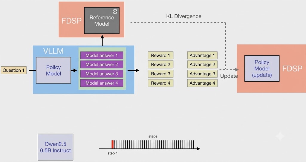
The GRPO approach to updating a policy involves sampling a group of model completions for the same prompt or query, \(q\). Each completion receives a reward. All the rewards in that group are normalized.

If a rollout is better than the group average, its advantage is positive. If a rollout is worse than the group average, its advantage is negative.

Since rewards are a blunt tool, we use advantages

\[\hat{A}_i = \frac{r_i - \mu_r}{\sigma_r + \epsilon}\]

where

\[\mu_r = \frac{1}{G} \sum_{i=1}^{G} r_i\]

\[\sigma_r = \sqrt{\frac{1}{G} \sum_{i=1}^{G} (r_i - \mu_r)^2}\]

When sampling a group of completions, we want their responses to be as diverse as possible. This is controlled by the temperature parameter of the language model.

The advantage \(\hat{A}_i\) is sequence-level and uses the mean (\(\mu_r\)) and standard deviation (\(\sigma_r\)) of the rewards within that specific group:

GRPO Objective Function

The GRPO loss function for all tokens is

\[\mathcal{L}_{GRPO}(\theta) = \frac{1}{G} \sum_{i=1}^{G} \frac{1}{|o_i|} \sum_{t=1}^{|o_i|} -\left[ \min\left(\rho_t(\theta)\hat{A}_i, \text{clip}\left(\rho_t(\theta), 1-\epsilon, 1+\epsilon\right)\hat{A}_i\right) - \beta \mathbb{D}_{KL}(\pi_\theta \| \pi_{\theta_{ref}})\right]\]

where

\[\rho_t(\theta) = \frac{\pi_\theta(o_{i, t}|q, o_{i, <t})}{\pi_{\theta_{old}}(o_{i, t}|q, o_{i, <t})}\]

\[\mathbb{D}_{KL} = \exp\left(\log \pi_\theta(o_{i, t}|q, o_{i, <t}) - \log \pi_{\theta_{ref}}(o_{i, t}|q, o_{i, <t})\right) - \left[\log \pi_\theta(o_{i, t}|q, o_{i, <t}) - \log \pi_{\theta_{ref}}(o_{i, t}|q, o_{i, <t})\right] - 1\]

\(\pi_{\theta_{old}}\): The state of trainable policy \(\pi_\theta\) before current trajectory rollouts are sampled. Outputs are generated using \(\pi_{\theta_{old}}\). We perform multiple gradient updates on \(\pi_\theta\) using the same batch of sampled trajectories. \(\pi_\theta\) starts to diverge from \(\pi_{\theta_{old}}\). It is updated to match \(\pi_\theta\) every time new completions are sampled from the environment.

\(\pi_{ref}\): The base model checkpoint. It remains fixed across the entire RL training run.

Worked Example – Update for a single group

1. Given a query \(q\), generate \(G\) responses to the query \(\pi_{old}(q) \to \{y_i\}_{i=1}^G\).

2. Compute Advantage values for each of the \(G\) responses. \[\hat{A}_i = \frac{r_i - \mu_r}{\sigma_r + \epsilon}\]

3. To compute GRPO Loss for a particular group, we compute the following for all tokens: \[\mathcal{L}_{GRPO} = -\frac{1}{G} \sum_{i=1}^{G} \sum_{t=1}^{|o_i|} \min[\rho_t(\theta)\hat{A}_i, \text{clip}(\rho_t(\theta), 1-\epsilon, 1+\epsilon)\hat{A}_i] - \beta \mathbb{D}_{KL}(\pi_{\theta} || \pi_{\theta_{ref}})\]

where \[\rho_t(\theta) = \frac{\pi_{\theta}(o_t | o_{i,<t}, q)}{\pi_{\theta_{old}}(o_t | o_{i, <t}, q)}\]

Let \(G=2\) and the query be \(q=\) “What is the capital of France?”

Let the responses being considered be

\(o_1\): “It is London”

\(o_2\): “The capital of France is Paris”

Let the advantage values associated with responses be

\(\hat{A}_1 = -1\), \(\hat{A}_2 = 1\).

Set \(\epsilon = 0.01\).

Further remarks before computing the ratio:

1. At first, when \(\pi_{\theta_{old}} = \pi_{\theta}\), the ratio will be 1. To avoid being trivial, we will assume \(\pi_{\Theta_{old}}\) has been trained for some iterations so it yields a different softmax probability

2. Actual softmax values will be simulated for illustration

3. We omit computing the KL divergence for simplicity

Consider the simplified ratio sum for response \(1, o_1\). Note: for this example, the token-level ratio \(\rho_t( \theta )\) is evaluated independently for each token \(t\) before averaging

\[\sum_{t=1}^{|o_1|} \rho_t(\theta) = \sum_{t=1}^{|o_1|} \rho_t(\theta) = \rho_1(\theta) + \rho_2(\theta) + \rho_3(\theta)\]

The tokens are \(o_{11}=\text{It}, o_{12}=\text{is}, o_{13}=\text{London}.\)

The ratio is

\(\rho_1(\theta) = \frac{\pi_{\theta}(o_{11}|q)}{\pi_{\theta_{\text{old}}}(o_{11}|q)} = \frac{0.05}{0.15} = \frac{1}{3}\)

\(\rho_2(\theta) = \frac{\pi_{\theta}(o_{12}|q, o_{11})}{\pi_{\theta_{\text{old}}}(o_{12}|q, o_{11})} = \frac{0.07}{0.28} = \frac{1}{4}\)

\(\rho_3(\theta) = \frac{\pi_{\theta}(o_{13}|q, o_{11}, o_{12})}{\pi_{\theta_{\text{old}}}(o_{13}|q, o_{11}, o_{12})} = \frac{0.03}{0.36} = \frac{1}{12}\)

Substitute in minimum. This Advantage for this response is \(\hat{A}_t = \hat{A}_1 = -1\)

\(\min [\rho_t(\theta) \hat{A}_t, \text{clip}(\rho_t(\theta), 1-\epsilon, 1+\epsilon)\hat{A}_t]\)

\(\min [\rho_1(\theta)(-1), \text{clip}(\rho_1(\theta), 1-0.01, 1+0.01)(-1)]=\min [\frac{1}{3}(-1), \text{clip}(\frac{1}{3}, 0.99, 1.01)(-1)] = -\frac{1}{3}\)

\(\min [\rho_2(\theta)(-1), \text{clip}(\rho_2(\theta), 1-0.01, 1 + 0.01)(-1)]= \min [\frac{1}{4}(-1), \text{clip}(\frac{1}{4}, 0.99, 1.01)(-1)] = -\frac{1}{4}\)

\(\min [\rho_3(\theta)(-1), \text{clip}(\rho_3(\theta), 1 - 0.01, 1 + 0.01)] = \min [\frac{1}{12}(-1), \text{clip}(\frac{1}{12}, 0.99, 1.01)] = -\frac{1}{12}\)

Average across tokens

\[\frac{1}{|o_i|} \sum_{t=1}^{|o_i|} \min [\rho_t(\theta) \hat{A}_t, \text{clip}(\rho_t(\theta), 1-\epsilon, 1+\epsilon)\hat{A}_t] = \frac{1}{3} [-\frac{1}{3} + -\frac{1}{4} + -\frac{1}{12}] = -\frac{2}{9}\]

Next, we do the same for response 2

\(o_2 = \text{"The capital of France is Paris"}\).

The tokens are denoted

\(o_{21} = \text{The}, o_{22} = \text{capital}, o_{23} = \text{of}, o_{24} = \text{France}, o_{25} = \text{is}, o_{26} = \text{Paris}\)

The ratios (truncated) are

\(\rho_1(\theta) = \frac{\pi_{\theta}(o_{26}|q, o_{21}, \cdots, o_{25})}{\pi_{old}(o_{26}|q, o_{21}, \cdots, o_{25})}\)

\(\cdots\)

\(\rho_6(\theta) = \frac{\pi_{\theta}(o_{26}|q, o_{21}, \cdots, o_{25})}{\pi_{old}(o_{26}|q, o_{21}, \cdots, o_{25})}\)

Skipping to the sum across tokens. The Advantage for this response is \(\hat{A}_t = \hat{A}_2 = 1\)

\[\frac{1}{|o_i|} \sum_{t=1}^{|o_i|} \min [\rho_t(\theta) \hat{A}_t, \text{clip}(\rho_t(\theta), 1-\epsilon, 1+\epsilon)\hat{A}_t] = \frac{1}{6}\]

Once we have processed the tokens in every response, we average across every response in the group (we omit the KL divergence for simplicity). Since we have 2 responses in the group, we sum and divide by 2.

\[\frac{1}{2} [-\frac{2}{9} + \frac{1}{6}] = \frac{1}{2} [-\frac{4}{18} + \frac{3}{18}] = \frac{1}{2} [-\frac{1}{18}] = -\frac{1}{36}\]

Rolling up to Batch Level

The defined GRPO loss was for all group responses for a single prompt/query. However, in a batch we have many prompts. To compute a loss over a batch, we compute the average again.

\[\mathcal{L}_{Batch} = \frac{1}{B} \sum_{b=1}^{B} \mathcal{L}_{GRPO}\]

Reinforcement Learning with Verifiable Rewards (RLVR)

In practice we use a training approach like RLVR. In RLVR, the reward is produced by a deterministic checker vs a learned reward model. For instance, given a math problem, a checker can compare the final answer vs known answer.

A model can generate many candidate solutions to a prompt and receive reliable signal without human labels for every response. RLVR applies when correctness is objectively verifiable. For more open-ended problems we require learned reward models, preference data, human evaluation or other alignment signals.

Practically speaking; we use verifiers where they are reliable and use preference signals where the target behaviour is not mechanically checkable.

A RLVR training run should be monitored with more than average reward. Average reward can rise while other behaviours degrade. E.g response length may increase but correctness may not. Useful monitoring metrics measure all aspects of desirable responses such as mean reward, pass rate, response length, KL divergence from reference policy, invalid format rate, duplicate output rate and reward variance within groups.

Practical Considerations

When performing model improvements via GRPO, we require 3 copies of the language model: 1. A frozen copy of the reference language model 2. The policy language model which is updated via GRPO 3. The policy language model which is used to generate rollouts for a given input \(q_i\). Typically served via vLLM.

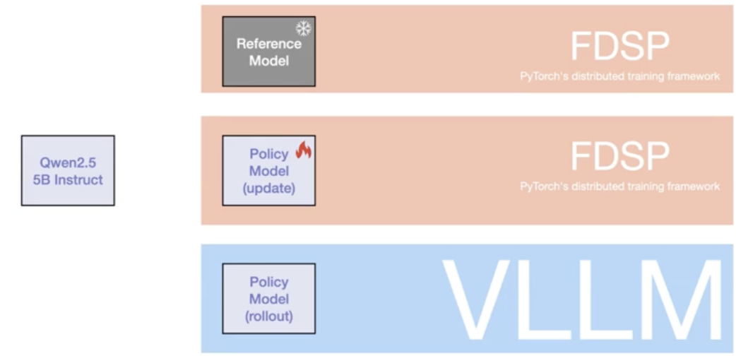
At every step, we have the following process