Just Go with the Flow

Recently, I’ve been down the rabbit hole of generating videos. I’m astonished by how these video generation models can produce realistic videos. In my ongoing study of them, I’ve learned that many of them have been trained using a paradigm of flow matching. This post is a (relatively) calculus free, ML first look into flow matching.

The goal is to make the key ideas clearer and to understand the training and inference paradigm for the latest generation if image and video models. In future I will hope to add to this from the point of view of mathematical theory and include some code examples. That being said, there are some mathematical fundamentals that have to be reviewed before this can make sense. Let’s begin!

Vector Fields

A vector field on 2 or 3 dimensional space is a function \(\vec{F}\) that assigns to each point \((x,y)\) or \((x,y,z)\) a vector given by \(\vec{F}(x,y)\) or \(\vec{F}(x,y,z)\).

The standard notation for the function \(\vec{F}\) is: \[\vec{F}(x,y) = P(x,y)\vec{i} + Q(x,y)\vec{j}\] where \(\vec{i} = [1,0]^T\), \(\vec{j} = [0,1]^T\).

Example 1: Consider \(\vec{F}(x,y) = -y\vec{i} + x\vec{j}\). at \((\frac{1}{2}, \frac{1}{2})\) we have

\[\vec{F}(1/2, 1/2) = -1/2\vec{i} + 1/2\vec{j} = [-1/2, 1/2]^T\]

at \((\frac{3}{2}, \frac{1}{4})\) we have \[\vec{F}(3/2, 1/4) = -1/4\vec{i} + 3/2\vec{j} = [-1/4, 3/2]^T\]

at \((1/2, 1/2)\) we plot the vector \(-1/2\vec{i} + 1/2\vec{j}\) at \((3/2, 1/4)\) we plot the vector \(-1/4\vec{i} + 3/2\vec{j}\)

If we plotted this we might see:

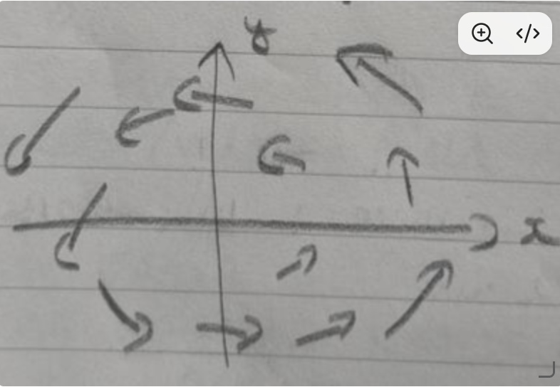
A vector field can also be denoted as \(\vec{v}(x,y)\) or \(\vec{v}(x,y,z)\).

A vector field can also be called a velocity field, this is inherited from fluid dynamics. If \(\vec{v}(x,y,z)\) is the velocity of a moving fluid at position \((x,y,z)\) then \(\vec{v}\) is called a velocity field.

Flow Matching Basics

Given a data distribution \(p_1\) on \(\mathbb{R}^d\) and a base noise distribution \(p_0 = \mathcal{N}(\mathbf{0}, I_d)\), we want a time dependent vector field \[v_{\theta}(\textbf{x}, t): \mathbb{R}^d \times [0,1] \to \mathbb{R}^d\] Such that solving \[\frac{d\textbf{x}}{dt} = v_{\theta}(\textbf{x}, t), \quad \textbf{x}(0) \sim p_0\] produces \(\textbf{x}(1) \sim p_1\).

For a given position at time t, \(v_{\theta}\) tells us how much we must move the point via an output offset vector at time t. \(v_{\theta}\) defines a vector over all positions \(\textbf{x}_t\).

Linear Probability Path

For a pair \((\textbf{x}_0, \textbf{x}_1)\) sampled from \((p_0, p_1)\), define the conditional path \[\textbf{x}_t = (1-t)\textbf{x}_0 + t\textbf{x}_1, \quad t \in [0,1]\] The velocity is a constant vector, the line segment is traversed at uniform speed \(||\textbf{x}_1 - \textbf{x}_0||\)

Marginalizing Over \((\textbf{x}_0, \textbf{x}_1)\) gives the marginal distribution of \(\textbf{x}_t\), denoted \(p_t\). Since \(\textbf{x}_0 \sim \mathcal{N}(\textbf{0}, I_d)\) and \(\textbf{x}_1 \sim p_1\) are independent, the conditional distribution of \(\textbf{x}_t\) given \(\textbf{x}_1\) is \[\textbf{x}_t | \textbf{x}_1 \sim \mathcal{N}(t\textbf{x}_1, (1-t)^2 I_{d})\]

This is a Gaussian centered on \(t\textbf{x}_1\) with variance \((1-t)^2\). As \(t \to 1\), variance \(\to 0\) and \(\textbf{x}_t\) concentrates on \(\textbf{x}_1\).

In other words, the probability concentrates on \(\textbf{x}_1\) as \(t \to 1\).

A probability path is a continuous sequence of distributions from \(t=0\) to \(t=1\), denoted \(p_t\). Each \(p_t\) is a probability distribution. For a fixed pair (\(\textbf{x}_0\), \(\textbf{x}_1\)), flow matching aims to move a noise point \(\textbf{x}_0\) along a straight line until it arrives to \(\textbf{x}_1\).

\[\textbf{x}_t = (1-t)\textbf{x}_0 + t\textbf{x}_1\]

At \(t=0\), \(\textbf{x}_t = \textbf{x}_0\) and we have Gaussian noise. At \(t=1\), \(\textbf{x}_t = \textbf{x}_1\) we have a real data sample. At \(0<t<1\), \(\textbf{x}_t\) lies along the line segment connecting \(\textbf{x}_0\) & \(\textbf{x}_1\). If we average over all noise-data pairs, the distribution of \(\textbf{x}_t\) interpolates between \(p_0\) & \(p_1\).

If we differentiate along the line segment:

\[\frac{d\textbf{x}_t}{dt} = -\textbf{x}_0 + \textbf{x}_1 = \textbf{x}_1 - \textbf{x}_0\]

More formally, let \(p_0\) be a probability distribution on \(\mathbb{R}^d\) that we can sample from. A good example is the Gaussian distribution.

\[p_0 = \mathcal{N}(\textbf{0}, I_d)\]

Let \(p_1\) be a data distribution, it can be the distribution of images or videos. To generate new images, we’d like to sample from \(p_1\) but we don’t know its analytic form. But we do have samples from \(p_1\) - \(\textbf{x}_i \sim p_1\).

The Goal of Flow Matching

Given a datapoint \(\textbf{x}\), sampled from a Gaussian, we want to learn a time varying vector-field such that it informs us how much we should move \(\textbf{x}\) (at time \(t\)) via an offset vector \(\Delta\textbf{x}\). We want to move \(\textbf{x}\) to be closer to a point \(\textbf{x}'\) that could be sampled from a target distribution - in our case \(p_1\). The goal of flow matching is to learn this time varying vector/velocity field from data.

Geometrically, imagine a random scattering of points in \(\mathbb{R}^d\). These look like they’ve been sampled from a Gaussian. We want to move these points, on a time schedule, such that at the end of this process we have a different topology of points. If we have trained well, the topology of data points resemble a sample from \(p_1\).

Time dependent vector fields

A vector field that varies based on time can be described by: \[v: \mathbb{R}^d \times [0,1] \to \mathbb{R}^d\] For each fixed \(t\), we have an ordinary vector field on \(\mathbb{R}^d\) - the snapshot of vectors at time \(t\). As \(t\) varies, the snapshot changes.

At a given point \(x^*\), the field can vary in 2 independent ways: 1. Spatial variation: At a fixed time, the arrow at the given point is different from the arrow at a nearby point \(x^{*} + \delta x\). 2. Temporal variation: At a fixed location \(x^*\), the arrow at time \(t\) is different from the arrow at time \(t + \delta t\).

Conditional Flow Matching Loss

\[\mathcal{L}_{CFM}(\theta) = \mathbb{E}_{t \sim u(0,1), \textbf{x}_1 \sim p_1, \textbf{x}_0 \sim p_0}[||\textbf{v}_{\theta}(\textbf{x}_t, t) - (\textbf{x}_1 - \textbf{x}_0)||^2]\]

where \(\textbf{x}_t = (1-t)\textbf{x}_0 + t\textbf{x}_1\). In practice we end up computing MSE loss.

Training Loop

1. Given a mini-batch of real data
2. Sample real data: \(\textbf{x}_1 \sim p(\textbf{x})\)
3. Sample noise: \(\textbf{x}_0 \sim \mathcal{N}(\mathbf{0}, \mathbf{I})\). \(\textbf{x}_0\) is same shape as \(\textbf{x}_1\)
4. Sample time: \(t \sim U[0,1]\)
5. Build an intermediate state: \(\textbf{x}_t = (1-t)\textbf{x}_0 + t\textbf{x}_1\)
6. Compute loss: \(L = \|v_{\theta}(\textbf{x}_t, t) - (\textbf{x}_1 - \textbf{x}_0)\|^2\) and backpropagate

Example 2: Consider a \(2 \times 2\) image

\[\textbf{x}_1 = \begin{bmatrix} 0.8 & 0.2 \\ 0.1 & 0.9 \end{bmatrix}\]

Let \(\textbf{x}_0\) to be sampled noise

\[\textbf{x}_0 = \begin{bmatrix} -0.4 & 1.2 \\ 0.3 & 0.7 \end{bmatrix}\]

Let \(t=0.5\). Then we build \(\textbf{x}_t\)

\[\textbf{x}_{0.5} = (1-0.5) \begin{bmatrix} -0.4 & 1.2 \\ 0.3 & 0.7 \end{bmatrix} + 0.5 \begin{bmatrix} 0.8 & 0.2 \\ 0.1 & 0.9 \end{bmatrix}\]

\[\textbf{x}_{0.5} = \begin{bmatrix} 0.2 & 0.7 \\ 0.2 & 0.8 \end{bmatrix}\]

Compute target velocity \((\textbf{x}_1 - \textbf{x}_0)\) \[\textbf{x}_1 - \textbf{x}_0 = \begin{bmatrix} 0.8 - (-0.4) & 0.2 - 1.2 \\ 0.1 - 0.3 & 0.9 - 0.7 \end{bmatrix} = \begin{bmatrix} 1.2 & -1.0 \\ -0.2 & 0.2 \end{bmatrix} = v_{tgt}\]

Suppose our model predicts

\[v_{\theta}(\textbf{x}_t, t) = v_{\theta}(\textbf{x}_{0.5}, 0.5) = \begin{bmatrix} 1.1 & -0.9 \\ -0.3 & 0.5 \end{bmatrix} = v_{pred}\]

Compute residual

\[v_{\theta}(\textbf{x}_{0.5}, 0.5) - (\textbf{x}_1 - \textbf{x}_0) = \begin{bmatrix} -0.1 & 0.1 \\ -0.1 & -0.1 \end{bmatrix} = r\]

Compute the scalar loss & backpropagate to update \(\theta\) \[L = MSE(v_{pred}, v_{tgt}) = \frac{1}{n} \sum_{i=1}^{n} (v_{pred, i} - v_{tgt, i})^2\] \[L = \frac{1}{4} [(-0.1)^2 + (0.1)^2 + (-0.1)^2 + (-0.1)^2] = \frac{1}{4} [0.01 + 0.01 + 0.01 + 0.01]\] \[L = 0.01\]

Inference

During inference, we don’t know \(\textbf{x}_1\), so we use an ODE solver, the most popular of which is Euler steps

\[\textbf{x}_{t+\Delta t} = \textbf{x}_t + (\Delta t \times v(\textbf{x}_t, t))\]

1. Draw a new Gaussian noise step \[\textbf{x}_0 = \begin{bmatrix} -0.4 & 1.2 \\ 0.3 & -0.7 \end{bmatrix}\]
2. Set Euler steps to \(t=2\). Our step size is thus \(\frac{1}{t} = \Delta t = 0.5\)

Step 1: \(t=0 \rightarrow 0.5\)

Suppose the learned model returns \(v_0 = \begin{bmatrix} 1.2 & -1.0 \\ -0.2 & 1.6 \end{bmatrix}\)

Perform Euler update

\[\textbf{x}_{0.5} = \textbf{x}_0 + \Delta t v_0 = \begin{bmatrix} -0.4 & 1.2 \\ 0.3 & -0.7 \end{bmatrix} + 0.5 \begin{bmatrix} 1.2 & -1.0 \\ -0.2 & 1.6 \end{bmatrix}\]

\[\textbf{x}_{0.5} = \begin{bmatrix} 0.2 & 0.7 \\ 0.2 & 0.1 \end{bmatrix}\]

Step 2: \(t = 0.5 \to 1\).

Let the model predict \[v_{0.5} = \begin{bmatrix} 1.2 & -1.0 \\ -0.2 & 1.6 \end{bmatrix}\]Update\[\textbf{x}_1 = \textbf{x}_{0.5} + 0.5 v_{0.5}\]

\[= \begin{bmatrix} 0.2 & 0.7 \\ 0.2 & 0.1 \end{bmatrix} + 0.5 \begin{bmatrix} 1.2 & -1.0 \\ -0.2 & 1.6 \end{bmatrix} = \begin{bmatrix} 0.8 & 0.2 \\ 0.1 & 0.9 \end{bmatrix}\]

In practice, we use 20-50 Euler steps during inference.

Latent Flow Matching

Flow matching operates on any continuous state \(\mathbf{x} \in \mathbb{R}^d\). In practice, models in production don’t operate in original image/video space, it is too high dimensional. Instead it operates in a learned latent space. Before building a model using flow matching on images, for example, we learn a compressed representation.

If we find a mapping \(E: \mathbb{R}^d \to \mathbb{R}^k\), \(k \ll d\) that preserves important information, we can run flow matching in \(\mathbb{R}^k\). In practice, a Variational Autoencoder (VAE) is used to project images (or videos) into a latent representation.

A latent \(\mathbf{z} \in \mathbb{R}^k\) contains learned features that emerge from training. The training & inference loops are minimally changed.

Training.

1. Sample an image \(\mathbf{x}_1\sim p_{\text{data}}\).
2. Encode: \(\mathbf{z}_1=E(\mathbf{x}_1)\).
3. Sample noise \(\mathbf{z}_0\sim\mathcal{N}(\mathbf{0},I_k)\) of the same shape as \(\mathbf{z}_1\).
4. Sample \(t\sim U[0,1]\).
5. Interpolate: \(\mathbf{z}_t=(1-t)\mathbf{z}_0+t\mathbf{z}_1\).
6. Compute velocity target: \(v_{\text{target}}=\mathbf{z}_1-\mathbf{z}_0\).
7. Predict: \(v_{\text{pred}}=v_\theta(\mathbf{z}_t,t,\mathbf{c})\) (with optional conditioning \(\mathbf{c}\)).
8. Loss: \(\mathcal{L}=\|v_{\text{pred}}-v_{\text{target}}\|^2\).

Inference.

1. Sample noise \(\mathbf{z}_0 \sim\mathcal{N}(\mathbf{0},I_k)\).
2. Integrate the ODE \(\frac{dz}{dt}=v_\theta(\mathbf{z},t,\mathbf{c})\) from \(t=0\) to \(t=1\).
3. Decode: \(\mathbf{x}=D(\mathbf{z}_1)\).

The VAE decoder translates latents back to image space, it (decoder) is called once after the flow matching process has concluded on the latents.

Model Architectures: How to build \(v_{\theta}\)

Flow matching is an objective, it does not specify the model structure. In practice, there are 2 popular model choices: 1. UNET 2. Diffusion Transformer (DiT)

What is key about these models is that it satisfies \[v_{\theta}: \mathbb{R}^d \times [0,1] \times \mathbf{c} \rightarrow \mathbb{R}^d\]

where

\(\mathbb{R}^d\) is the state/position \([0,1]\) is time \(\mathbf{c}\) is conditioning (we will discuss later)

If the state is a \(C \times H \times W\) tensor, the output must be \(C \times H \times W\). The output must have the same Shape as the Input

Conditioning and Classifier Free Guidance

The flow matching setup thus far has been unconditional to generate a sample from the data distribution \(p_1\). Real models allow conditioning on a prompt. To accommodate this, our learned network can be denoted as \(v_{ heta}(\textbf{x}_t, t, \textbf{c})\) where \(\textbf{c}\) encodes conditional signal - commonly a text prompt embedded via CLIP.

There are 2 mechanisms involved: 1) Conditioning: The network sees \(\textbf{c}\) and adjusts its predicted velocity towards data samples from \(p_1\) matching the condition \(\textbf{c}\). 2) Classifier Free Guidance: At inference, combine conditional and unconditional predictions to amplify the effect of the condition.

The most common conditioning signal is a text Prompt embedded into a vector.

There are 3 common patterns to Plug condition \(\textbf{c}\) into the model network:

1. Cross Attention: Query the image tokens against \(\textbf{c}\).
2. Concatenation: Prepend/append the text tokens to the image tokens in a Transformer.
3. AdaLN module: Use a small Multilayer Perceptron (MLP) to turn \(\textbf{c}\) into scale/shift parameters for LayerNorm Layers. Common alongside cross-attention.

Suppose we have 2 versions of the model:

1. Conditional: \(v_{\theta}(\textbf{x}_t, t, c)\) - Predicts the velocity to reach data matching \(c\).
2. Unconditional: \(v_{\theta}(\textbf{x}_t, t, \phi)\) - Predicts the velocity to reach data in general, ignoring \(c\).

The difference \(v_{\theta}(\textbf{x}_t, t, c) - v_{\theta}(\textbf{x}_t, t, \phi)\) is the added push that conditioning provides. Classifier-free Guidance amplifies this difference: \[v_{guided}(\textbf{x}_t, t, c) = v_{\theta}(\textbf{x}_t, t, \phi) + w[v_{\theta}(\textbf{x}_t, t, c) - v_{\theta}(\textbf{x}_t, t, \phi)]\]

where \(w \ge 1\) is a guidance scale. having \(w > 1\) ensures the conditional direction is exaggerated beyond what the model itself predicts.

During training, we don’t train separate networks. Rather we occasionally drop the condition \(c\). For a given training example, with probability \(p_{drop} \in (0.1, 0.2)\), we replace \(\mathbf{c}\) with a null token \(\phi\).

The single network \(v_{\theta}\) learns to handle both cases. At inference, we evaluate the same network twice - once with the real \(\mathbf{c}\) and once with \(\phi\) and combine.

Geometrically, \[v_{\theta}(\textbf{x}_t, t, \phi)\]

can be thought of as velocity towards any plausible datapoint sampled from \(p_{1}\) and \(v_{\theta}(\textbf{x}_t, t, c)\) be the direction towards any plausible datapoint sampled from \(p_1\) consistent with \(c\). The difference vector points from generic data toward data satisfying \(c\).

Negative Prompts

Many models support a negative prompt \(\mathbf{c}^-\), which is a description of what we don’t want in the generated image. The guidance formula then becomes \[ v_{\text{guided}} = v_{\theta}(\textbf{x}_{t}, t, \mathbf{c}^{-}) + w[v_{\theta}(\textbf{x}_{t}, t, \mathbf{c}^+) - v_{\theta}(\textbf{x}_{t}, t, \mathbf{c} ^-)] \]

By subtracting the direction associated with the anti-prompt, we push the trajectory away from features described by \(\mathbf{c}^-\)

Extension to Video models: Video Flow Matching

A video is a spatiotemporal tensor: \[\textbf{x} \in \mathbb{R}^{T \times C \times H \times W}\]

where

\(T = \text{number of frames}\)

\(C = \text{number of channels (3 for RGB, more for latents)}\)

\(H, W = \text{spatial dimensions}\)

A high resolution video at \(T=48, H=W=720, C=3\) has dimension \[d = 48 \times 3 \times 720 \times 720 \approx 7.5 \times 10^7\] since this is prohibitively high, video generation almost always operates in a latent space.

Case Study: Wan 2.1

Wan 2.1, an open source model by Alibaba is a text to video system built on flow matching. A sketch of the inference pipeline:

1. Text encoding: A Prompt is transformed into a sequence of token embedding
2. Sample noise: \(Z_0 \sim \mathcal{N}(\textbf{0}, \textbf{I})\) with the shape matching the target video latent
3. Iterate Euler steps (typically 50); at each step:
   • Concatenate text & video latent to kens
   • Pass through a Diffusion Transformer (DiT) with spatio temporal attention
   • The DiT outputs a velocity of the same shape as the video latent
   • Apply Classifier-free guidance
   • Take an Euler step
4. Decode: Pass the final \(\mathbf{z}_1\) through the video VAE decoder to obtain pixels.

Example 3: 2 frame video inference pass

Suppose the trained network happens to return the exact target velocity at every point (idealised). Use 2 Euler steps of \(\Delta t=0.5\).

Start. \[ x_0=\left(\;\begin{bmatrix}-0.5 & 0.4\\ 1.0 & -0.2\end{bmatrix},\;\begin{bmatrix}0.3 & -0.7\\ -0.1 & 0.8\end{bmatrix}\;\right). \]

Step 1 (\(t=0\to 0.5\)). Network returns \[ v_0=\left(\;\begin{bmatrix}1.5 & -0.4\\ -1.0 & 0.2\end{bmatrix},\;\begin{bmatrix}-0.3 & 1.7\\ 0.1 & -0.8\end{bmatrix}\;\right). \]

Euler: \[ x_{0.5}=x_0+0.5\,v_0. \]

Frame 1: \[ \begin{bmatrix}-0.5+0.75 & 0.4-0.2\\ 1.0-0.5 & -0.2+0.1\end{bmatrix}=\begin{bmatrix}0.25 & 0.20\\ 0.50 & -0.10\end{bmatrix}. \]

Frame 2: \[ \begin{bmatrix}0.3-0.15 & -0.7+0.85\\ -0.1+0.05 & 0.8-0.4\end{bmatrix}=\begin{bmatrix}0.15 & 0.15\\ -0.05 & 0.40\end{bmatrix}. \]

Which matches the training example’s \(x_{0.5}\).

Step 2 (\(t=0.5\to 1\)). For a straight-line path the velocity is constant, so the network again returns the same vector. Update: \[ x_1=x_{0.5}+0.5\,v_{0.5}. \]

Frame 1: \[ \begin{bmatrix}0.25+0.75 & 0.20-0.20\\ 0.50-0.50 & -0.10+0.10\end{bmatrix}=\begin{bmatrix}1.0 & 0.0\\ 0.0 & 0.0\end{bmatrix}. \]

Frame 2: \[ \begin{bmatrix}0.15-0.15 & 0.15+0.85\\ -0.05+0.05 & 0.40-0.40\end{bmatrix}=\begin{bmatrix}0.0 & 1.0\\ 0.0 & 0.0\end{bmatrix}. \]

Both frames land exactly on their targets, and the “bright pixel” has moved from the top-left to the top-right — motion has been generated by the flow.

Interpretation of the result. The bright pixel’s trajectory in pixel space is:

• Frame 1: pixel \((0,0)\) has intensity 1.
• Frame 2: pixel \((0,1)\) has intensity 1.

The temporal dependence is entirely handled by the network’s spatiotemporal attention: it sees both frames at once and produces a joint velocity. If the network had been trained only on isolated frames, the two output frames would be uncorrelated random bright-pixel positions.